An Empirical Analysis of the Volatility Spillovers
between Commodity Markets, Exchange Rates, and
the Sovereign CDS Spreads of Commodity
Exporters
ABSTRACT:
In this paper, we investigate the volatility spillovers between Commodities, Foreign Exchange Rates, and the CDS Spreads of several commodity exporting nations from 2012 to late 2021, and how COVID-19 affects these results. Utilising five country-specific VARs in the Diebold and Yilmaz (2012) framework for Australia, Peru, Chile, Colombia and Russia, we discover volatility spillovers from FX to CDS, Commodities to CDS, and
CDS to Gold. We also identify model efficiencies, improvements, and areas where this topic can be developed further in the interest of portfolio risk management and policy.
NAME: Alfie J. Fox-Heaton
SUPERVISOR: Kevin C. Lee
STUDENT ID: 20373244
DATE: 30/08/2022
This Dissertation is presented in part fulfilment of the
requirement for the completion of an MSc in the School of
Economics, University of Nottingham. The work is the sole
responsibility of the candidate.
TABLE OF CONTENTS
1. INTRODUCTION ……………………………………………………………………………………………..
2. THEORETICAL LITERATURE REVIEW ……………………………………………………….
3. ECONOMETRIC LITERATURE REVIEW …………………………………………………….
4. APPLIED ECONOMETRIC LITERATURE REVIEW ……………………………………
5. DATA ………………………………………………………………………………………………………………
6. METHODOLOGY …………………………………………………………………………………………..
7. MODELS & RESULTS ……………………………………………………………………………………
8. DISCUSSION …………………………………………………………………………………………………..
9. CONCLUSION ………………………………………………………………………………………………..
10. REFERENCES ………………………………………………………………………………………………..
11. APPENDICES ………………………………………………………………………………………………….
1. INTRODUCTION
Throughout modern history and the development of nations into the 21st century, there has beena plethora of literature studying the role of natural resource abundance and in this paper, we investigate a specific phenomenon, first coined as the “resource curse” (Auty, 1993) in the applied to volatility transmission across financial markets. Such a phrase is most commonly used in the context of a nation-state possessing a significant quantity of natural resources which is both large relative to other producer countries (of that particular commodity) and accounts for a significant proportion of the country’s economic activity. The negative connotation attached to the term relates to how a seemingly positive geological attribute of a nation can breed various negative effects or embeds fragility into macroeconomies. The phenomenon often involves a self-fulfilling prophecy where investment is sucked up by the resource’s extractive industry, depriving the opportunity for the nation’s GDP and fiscal income to be more diversified, leading to greater volatility in revenues. Therefore, when commodity prices experience periods of high volatility nations, with large export dependencies on such commodities experience shocks through the terms of trade mechanism- which is an account of the import and export prices for particular commodities. Therefore, pricing shocks in commodities (those accounting for a significant amount of those for exports) propagate shocks through to output in the resource extracting sectors, which are then transmitted outward into the macroeconomy due to their size, significance, and interrelatedness with other industries. These are known as Commodity Terms of Trade (CToT) effects, and whilst this is a well researched area undertaken in both theoretical and empirical contexts (with the use of structural macroeconomic models) we find relatively little research applied to that of the financial markets in the context of volatility spillovers.
We, therefore, add discussion from structural macroeconomics into the context of financial market movements by utilising the Diebold and Yilmaz (2012) framework to investigate the volatility spillovers between various key financial instruments theoretically involved in, and affected by, the nature of CToT shocks. Those identified include Commodity Futures, Foreign Exchange Rates (FX), and Credit Default Swap (CDS) markets. With commodity prices being the driving force between the CToT shocks, their market is internationally traded via the use of financial derivatives such as forwards and futures, both publicly tradable and private (known as Over the Counter) but in the case of this paper, we use publicly known futures prices. We find sovereign CDS spreads to be a strong proxy for macroeconomic uncertainty (or instability) as they represent the price of insurance on sovereign bonds. As CDS contracts are also publicly tradable (but only amongst sophisticated investors and institutions), events which inject uncertainty and arouse speculation around an entity’s creditworthiness, result in increases in the price of such insurance (Wang et al., 2018). Financial market participants purchase such contracts for hedging (as they own the underlying bond) or even speculative purposes- one does not have to own an underlying bond to purchase CDS. Conversely, situations which result in the quashing of uncertainty around an entity’s creditworthiness such as a stable political situation, or a generally positive economic outlook will cause the price of such insurance to decrease through the same mechanism. FX markets also play a key role in the macroeconomic adjustment to CToT shocks as shock absorbers and are themselves a potential form of macroeconomic instability, they are therefore important to include in our volatility spillover analysis, allowing us to observe the spillovers from commodities to FX and from FX to CDS. We find this a particularly interesting area of research to expand upon for trading, investment management, risk management, and government policy. Although there is some existing applied literature in the context of return and volatility spillovers amongst CDS spreads and commodity markets, there is little discussion linking such studies to the macroeconomic theories we allude to, in addition to secondary studies of breaking down the model-generated time series spillovers and explaining differences amongst countries using cross-sectional data. We, therefore, differentiate from the techniques used in the existing applied literature but also suggest where the literature can be taken in the future as part of larger studies of these financial volatility spillovers using the Diebold and Yilmaz (2012) framework.
2. THEORETICAL LITERATURE REVIEW
To understand the theoretical linkage between commodity price volatility and the volatility of
CDS spreads in commodity export-dependent countries, we first turn to the economic literature
on the resource course. The papers on such a topic are broad, but we identify two strands of the literature most relevant to our study that can be categorised into several different areas, principally those quantifying the shocks of commodity prices through the terms of trade mechanism and into fundamental macroeconomic variables, those investigating the role of such shocks in the context of sovereign credit health, and those focus on the institutional context within countries identified as possessing the resource curse. Firstly, we examine those papers
on Terms of Trade shocks before relating these findings to the sovereign risk literature and finally adding context by referencing the role of institutional factors.
The empirical literature on the macroeconomic effects of commodity price shocks overwhelmingly revolves around terms of trade shocks, and some of the early literature on this phenomenon includes that of the paper by Mendoza (1995). Inspired by the developments in developing countries after the Oil-price boom and bust in the 1970s-1980s and other commodity price rises during the 1980s which resulted in significant terms-of-trade shocks, the authors utilise an intertemporal Real Business Cycle (RBC) model to investigate the dynamics between these shocks and business-cycles in a wide array of economies. They design the transmission mechanism between terms of trade shocks with the inclusion of variables such as the cost of imports and the purchasing power of exports. The paper’s findings indicate that terms-of-trade shocks account for approximately 50% of the variance in GDP. Such results appear questionable, especially when the wide array of countries used is considered.
In a similar study, Kose (2002) investigates the role of global price shocks on a sample of small open economies, also utilising a multi-sector RBC-derived model, and extends the work of Mendoza (1995) with a more sophisticated design of sectors where production inputs are concerned, therefore accounting for both the import and export commodity price channels. The author argues this “limits the substitution effects across different types of factors and reduces the volatility of primary sector output. This, in turn, decreases the volatility of aggregate output, and helps the model to generate realistic volatility properties.” (pp. 301). Despite being a
sensible approach to limit the role of commodity terms of trade shocks and test the unrealistic results generated by Mendoza (1995), the paper still finds that global price shocks explain the variation of 88% of output and 90% of investment when both the import and export channels are considered (pp.301). Broda and Tille (2005) analyse the commodity terms of trade shocks across 75 developing countries and the increased output volatility arising from such shocks by utilising a VAR model and impulse response functions to simulate the “dynamic paths of real GDP, the real exchange rate, consumer prices, and the terms of trade” (pp. 3). The authors specifically test the hypothesis that countries with flexible exchange rate regimes will be more resilient to commodity price shocks, finding those nations with flexible exchange rate regimes suffer fewer volatile contractions in output. This is a logical finding as pegging a currency to that of another requires monetary authorities to sell the foreign currency it is pegged to in return for the purchase of their domestic currency in the event of a negative terms of trade shock ceteris paribus- and the contrary in the event of positive terms of trade shock. The former case dries up investment in the domestic economy as interest rates naturally rise as a result (due to contraction in the domestic currency) in addition to allowing export prices to adjust and retain their competitiveness, with both implications leading to subsequently higher output variance.
Kaminsky (2010) analyses the impact of commodity prices in various commodity-exporting countries as this can potentially lead to complacently loose fiscal policy due to a boom in tax revenues, thus embedding a degree of fragility into the fiscal condition of such countries. After testing such a hypothesis, they find that booms in the terms of trade do not necessarily lead to such a fiscal response, as in OECD and upper-middle income countries a Keynesian (countercyclical) spending is undertaken whilst in OECD and low-income countries acyclical (uncorrelated) policy spending is undertaken. That being said, Kaminsky (2010, pp. 40) found
that during episodes of capital flows, lower-middle-income countries and (to a lesser extent) upper-middle-income countries undertake procyclical spending, supporting the hypothesis confirmed by other papers signalling fiscal incompetence during commodity booms. Therefore, the response by governments is heterogenous by the idiosyncrasies of nations.
Fornero, Kirchne, and Yany (2014) analyse the terms of trade shocks on investment in commodity-exporting countries, with a focus on Chile and small open economies primarily involved with exporting commodity metals by using a SVAR in addition to a bespoke DSGE model built for Chile. Such economies included those of Australia, Canada, Chile, New Zealand, Peru and South Africa. Analysing cross-country patterns, the authors find that
commodity price increases drive investment into the resource extracting sectors which spill into the non-commodity sectors- confirming previous theories of the resource curse effects. They add that such spillovers depend on the magnitude and longitude of the shock and that shocks were less severe in nations with free-floating exchange rate regimes.
Schmitt-Garohe and Uribe (2018) criticise the existing literature due to the bulk of the consensus that commodity terms of trade shocks through the export channel are overwhelmingly derived from calibrated business cycles, and that their approach is based on country-specific SVARs arrives at a starkly different conclusion for the 38-country dataset utilised. The authors conclude that by using this alternative approach, terms of trade shocks through the commodity export price channel alone generate only 10% of output variation and demonstrate the contrasting results between business-cycle and SVAR models by estimating a three-sector business cycle model and its structural parameters.
In another paper Fernandez, Schmitt-Garohe and Uribe (2017) present findings on the effects of terms of trade shocks that challenge the bulk of the existent literature based on SVAR models with calibrated business cycle models by using panel estimates on 138 commodities in a dual price approach including commodity prices relevant to both domestic consumption and production, where previous literature had only focused on the latter. They conclude that by using multiple commodities and transmission routes, these shocks account for 33% of output variation on average, signalling that import prices play a greater role in terms CToT shocks. The two papers formulate the author’s views that the commodity export price channel alone produces far smaller variation in output than previously known and that the commodity import
price channel is an important driver of commodity terms of trade shocks- echoing the findings
of Kose (2002) albeit to a lesser extent.
Much of the debate around CToT shocks seeks to assess whether terms of trade movements are anticipated or not (and hence transmitted through to business cycle dynamics or not). Zeev, Pappa, and Vicondoa (2017) utilise a GVAR to assess the Commodity Terms of Trade shocks to the economies of various Latin American countries and ensure the macroeconomic impacts of news shocks to the Terms of Trade of these countries are captured, then concluding that CToT shocks explain circa 50% of output variation when news shocks are accounted for, warning that papers such as Schmitt-Garahe and Uribe (2018) will greatly underestimate export oriented CToT effects when not accounting for news effects.
Roch (2019) utilises a heterogenous panel SVAR to analyse the macroeconomic responses to commodity price shocks across 22 commodity-exporting economies. The author finds that such shocks account for approximately 30% of output variance as opposed to earlier studies which find shocks explaining only around 10% of output variation. Although this is true Roche (2019) notes that there was great heterogeneity in macroeconomic responses to such shocks across the sample of 22 countries. Different to other studies on commodity price shocks, the use of panel SVAR is justified to study how responses to shocks vary by country characteristics. The author finds that “exchange rate flexibility, inflation targeting regimes and fiscal rules” (pp. 437) ensure greater macroeconomic resilience to commodity price shocks. Al-Sadiq, Bejar, and Otker (2021) assess the impact of commodity price shocks on Caribbean countries in the context of their exchange rate regimes. The study was motivated by theoretical groundings that commodity exporters with flexible exchange rates, as opposed to those with pegged regimes (where the currency is fixed relative to that of the US dollar for example), will be able to better adjust to commodity shocks (floating exchange rates are a stabilisation mechanism for macroeconomic shocks), however, the implementation of such exchange rate regimes have been cited to have complex trade-offs and yield uncertain results in economies without developed financial markets. Similar to the study by Roch (2019), the authors utilise a panel VAR and also find that economies with great exchange rate flexibility were more resistant to commodity price shocks. Specifically, these economies were able to adjust and recover more rapidly to such shocks in addition to achieving higher economic growth rates on average than those with pegged exchange rate regimes.
With the robust theoretical background behind CToT shocks, it is no surprise that there has also been the development of the sovereign debt literature on the resource curse. Dauvin (2016) investigates the role of commodity prices in the perception of sovereign risk in financial markets across 22 emerging market economies through the use of credit spreads. Their findings link the literature on sovereign debt to those of actively traded financial markets as high commodity prices for exporters mean that (through the CToT mechanism) the credit constraint for such nations is relaxed due to the fiscal windfalls received, allowing better debt management throughout booms. Although the terms of trade literature find commodity price shocks materially affect output, the authors conclude that “high variations in commodity prices are not particularly reflected in the way markets assess sovereign risk” (pp. 1).
Hamann et al. (2018) assess the relationships between the fluctuations in Oil prices, the effects these have on the macroeconomic environment of Oil-exporting economies, and subsequently, their sovereign risk by creating an open-economy model with incomplete financial markets whilst allowing the optimal level of Oil extraction and sovereign risk to interact. The authors conclude that whilst sovereign risk decreases as Oil producer size increases due to the nation’s ability to make payments on its debt, autarky becomes more attractive when the amount of Oil reserves increases which therefore increases the sovereign risk. Using a panel Vector Error Correction Model (VECM), Ampofo et al. (2021) analyse both the long-run and causal causation between natural resource rents and public debt. With the dataset consisting of 17 commodity-exporting economies from 1991 to 2017, the findings indicate that in the long-run earnings from natural resource exports are positively related to public debt whilst in the short run they are negatively related. The authors note that this implies “overdependence on total natural resource rents affects public debt sustainability of the panel countries if effective fiscal and economic management policies are disregarded”. Therefore, institutional quality plays a major role and that nations with strong institutions can take advantage of their natural resources in a way that is fiscally and economically sustainable to not increase sovereign default risk.
Ghecham (2020) also approaches the relationship between the commodities and their exporters under the context of the resource curse by analysing the role of Oil reserve abundance in the debt overhang of countries. By using a Structural Equation Model (SEM), their results show a positive correlation between inefficient government investments in the resource extracting sectors and weak institutions with such investments being typically procyclical, similar to the findings of Kaminsky (2010), and that the combination of debt accumulation from inefficient investments with lack of income diversification can lead to countries being more vulnerable to export CToT shocks, resonating with the conclusion of Ampofo et al. (2021). The findings of Robinson et al. (2006) show that such misallocations of resources may be due to elected officials placing an excessively high discount rate on the future, driven by the electoral process and that despite resultant income volatility, the subsequent windfalls from resource booms provide them with resources to influence elections.
3. ECONOMETRIC LITERATURE REVIEW
The bulk of the volatility modelling literature in financial economics began with the seminal paper on Auto-Regressive Conditional Heteroskedasticity (ARCH) by Engle (1982). Such a model aimed to simply take the lagged squared errors in addition to a constant to explain the variance at time t. Following this, many improvements were made such as the Generalised ARCH (GARCH) model introduced by Bollerslev (1987), in addition to variants which accounted for fat-tailed distributions and asymmetric responses to price changes which better model the asymmetric response of volatility (Brownlees et al., 2011). These models were not able to capture volatility spillovers effectively without major modifications, however.
Although this class of models was useful in explaining asset volatility, what was missing was a specialised class of models, designed specifically the modelling multivariate volatility relationships. This is where the advent of Multivariate GARCH (M-GARCH) models pushed the literature further to achieve this beginning with the Constant Conditional Correlation GARCH (CCC-GARCH) model by Bollerslev (1990). Such a model sought to assess the relationship between two or more asset market volatilities, assessing their respective correlations and covariances and relying on the residuals from the conditional mean model being constant over time. The downfall with the CCC-GARCH however is that correlation is not constant over time. Seeking to improve on this, a variety of M-GARCH models were developed to model time-varying correlations and covariances to reflect this reality in asset markets. The most notable of these is the Dynamic Conditional Correlation GARCH (DCC GARCH) introduced by Engle (2002). The advantage of this approach is that it does not only reproduce realistic time-varying correlations and covariances characteristic of reality and that the estimated volatility parameters produced by the model are identical to the univariate GARCH models- dependent on what variant is used. The DCC-GARCH achieves this by modelling the univariate volatilities and then computing the conditional covariances as nonlinear functions of the conditional variances by weighting these by conditional quasicorrelation parameters. Tsu and Tsui (2002) develop a very similar, albeit lesser used, M-GARCH variant coined as the Varying Conditional Correlation GARCH (VCC-GARCH) which also allows the correlations and covariances to be time-varying using similar techniques possessing the same flexibility as the DCC variant. Although the conditional correlation subset of the M-GARCH class of models can potentially indicate volatility spillovers where covariances and correlations increase at a given time, this does not indicate causal spillovers, nor does it indicate the direction from which the spillovers originated.
For this reason, the bulk of the literature utilises the earlier model developed by Engle and Kroner (1995) therefore known as the BEKK-GARCH after the names of the authors. This model was not only able to capture the significance of any time-varying correlations but also the causal significance of volatility spillovers in addition to their specific directional influence. Despite this, the model had some major drawbacks such as the widely
cited inaccurate estimates of time-varying correlations and covariances in addition to not being parsimonious and generating many parameters to estimate which often led to the optimisation convergence failure of such a model when a large data set was utilised. Although the BEKK GARCH suffered from these drawbacks, it was one of the only M-GARCH models capable of directly testing causal directional volatility spillovers and was (and is, therefore) still a popular method used throughout the literature on volatility spillovers across a variety of asset classes. Because of these drawbacks, however, it is common that the model is accompanied by the DCC-GARCH which was found to produce superior estimates of both time-varying covariances and correlations as a cross-checking mechanism.
The remainder of the literature on volatility spillovers overwhelmingly revolves around Vector Autoregressions (VARs) principally using Forecast Error Variance Decompositions (FEVDs) computed by using the Moving Average representation of the estimated process and using this as the cut-off point at which the stochastic shocks are captured- and the forecast error resulting from them. Modelling return and volatility spillovers between numerous global equity indices, Diebold and Yilmaz (2008) use a novel approach, manipulating the FEVDs to create an index of spillovers. In the approach of volatility modelling, they take inspiration from Engle and Ito (1990) who embed GARCH estimated volatilities into a VAR system to investigate the global volatility transmission patterns across foreign exchange rates. Instead of using a GARCH method to estimate volatility, however, they utilise estimation methods by Garman and Klass (1980) relying on Open, High, Low, and Close (OHLC) pricing data. The spillover indices did not involve directional metrics of return and volatility spillovers though, which are critical in our analysis of assessing the volatility spillovers between commodities, FX, and CDS spreads.
The most fatal issue with this approach however is that it utilised the standard VAR framework which requires the assumption of ordering through Cholesky decomposition and a choice of a lower triangular matrix for the variance-covariances in the FEVD computations. In the context of financial market spillovers, this assumption is a fragile foundation for this analysis when many assets are often traded simultaneously. Despite possessing a theoretical foundation for the order of causality, it is therefore difficult to justify the order of this between the variables when simultaneous trading may mean simultaneous information sets.
In a majorly influential paper, Diebold and Yilmaz (2012) extend their previous paper in two ways. Firstly, they use the generalised FEVDs (GFEVDs) as introduced by Koop et al. (1996) as well as Pesaran and Shin (1998) denoted as the KPPS framework, and secondly, they add several other spillover indices aside from the total index of spillovers introduced in Diebold and Yilmaz (2008). The introduction of GFEVDs from the KPPS framework overcomes the issues with the orthogonalization of shocks in the standard VAR models and instead assumes shocks are contemporaneously correlated when hit by an overarching shock to the model, then capturing the covariances between assets to capture the GFEVDs.
Hyeongwoo (2009) however, criticises this approach and instead argues that the KPPS framework (despite being built to sidestep the extreme ordering assumptions) imposes extreme restrictions on the model and can lead to potential misinterpretation in structural economic models. Although this criticism warrants some credit, it is important to note that Diebold and Yilmaz (2008) also tested the results of the FEVDs across ordering combinations for the orthogonalized variant and did not find any significant differences, though due to the different combinations that can be specified in a lower triangular matrix such results of the comparison are precarious which is especially the case when the quantity of N variables increases- making it impractical to obtain the appropriate number of model combinations. Additionally, the nature of financialised nature of our variables in the model means that even if this was true, simultaneous information sets would make orthogonalization infeasible as alluded to previously. The additional spillover indices also make directional examinations of spillovers possible as opposed to just the aggregate bi-directional spillovers in a given VAR system.
These include total directional spillovers from and to N-1 other variables for a given variable, which allows us to then compute net spillovers between a variable and the rest of the system where gross spillovers do not provide much informational content for analysis in comparison. Moreover, the Diebold and Yilmaz (2012) framework also enables the computation of Net Pairwise spillovers between two variables which are instrumental in providing insights between CDS and Commodities (or FX). In a more recent paper, Diebold and Yilmaz (2014) introduce the network visualisation method in their series of GFEVD manipulations in VAR systems in addition to new metrics built to analyse the “connectedness” of markets. These methods would indeed be of great utility if we were to use a single VAR model for every variable in our study so that both intra-and inter asset contagion can be mapped. For example, relationships could also be analysed between specific commodities, FX rates, or CDS spreads to provide a richer analysis of where spillovers truly originate from as they may occur in sequences across markets. Although this is true our analysis involves country-specific approaches to test how findings differ from those of other papers in the applied literature and we suggest this technique is applied in larger studies.
4. APPLIED ECONOMETRIC LITERATURE REVIEW
After identifying the theoretical support for our investigation from the literature on CToTs and sovereign debt, as well as identifying various econometric techniques for spillover modelling in isolation, we turn to the applied literature on the analysis of commodity price spillovers and CDS spreads. Hooper (2015) uses a cross-sectional panel of data relevant to Oil and gas export dependent emerging market economies in analysing whether the reserves of Oil and gas themselves affect the CDS spreads of such countries. The author’s findings indicate that whilst Oil reserves lead to increases in CDS spreads (as a result of increased risk perceived by the financial markets), the effects of gas reserves are to the contrary, and decrease the CDS spreads. Moreover, Hooper (2015) finds significant interactions between institutional variables when introduced, and the results of which highlight the financial markets placing greater importance on political stability. This confirms other findings on the role of institutions in commodity terms of trade effects and sovereign risk, which are relevant for this topic but are not suitable for the scope of this time series spillover study.
Chuffart and Hooper (2019) then build on the work of Hooper (2015) to analyse the effects of Oil on the sovereign CDS spreads of both Russia and Venezuela by using a Markov-switching Time-Varying Transition Probabilities model (MSTVT) with the inclusion of other global and local factors such as nominal exchange rates. They find that Oil price returns have a statistically significant impact on the CDS spreads of Venezuela but for Russian CDS spreads, the nominal exchange rate is seen to play a greater role than the Oil price returns. It is important to note however that the methods used by Hooper (2015) as well as Cheuffart and Hooper (2019) are not trivial, nor are they spillover-enabled frameworks and therefore do not lend themselves to our branch of analysis.
Bouri et al. (2017) investigates volatility spillovers from commodities to sovereign CDS in seventeen emerging markets and six frontier markets using separate GARCH (Generalised Autoregressive Conditional Heteroskedasticity) models for each variable with an additional AR (Autoregressive) term so the conditional mean and variance of assets are modelled, then augmenting the model and using a Lagrange Multiplier (LM) test to formally assess spillovers.
The authors split the countries into their types of commodity export dependence and assess spillovers between their respective CDS spreads and the commodity indices most relevant to them. Although the paper demonstrates the significant transmission of volatility from commodity prices to sovereign CDS spreads in 10 of the Emerging Market countries, much of the transmission detected (through the rejection of their null hypotheses) occurred from commodity sub-indices which did not contain commodities that account for a significant proportion of their exports. The authors cite this as being due to the “financialization of commodities and the increased correlation between different commodities” (Bouri et al., 2017, pp. 163). Another important note to the methods used is that although they enable the statistical testing of causation-in-variance, they do not show how commodity spillovers vary across time with high frequency and only use sub-sampled data to achieve this.
In a later paper, Bouri et al. (2019) extend the methods in their earlier paper, this time focusing on BRICS countries (Brazil, Russia, India, China, and South Africa) and how Oil prices spill over into the sovereign CDS of such countries. They instead use a GARCH-quintile approach, measuring only the extreme volatility spillovers rather than all volatility spillovers, essentially testing the hypothesis of whether extreme volatility in commodity market prices causes extreme volatility in sovereign CDS spreads. Using data from January 2010 to August 2016, the authors conclude that the transmission of volatility from commodities to sovereign CDS varies under different volatility conditions and find that energy market volatility spillovers are only significant in the middle and upper quantiles of CDS volatility.
Sun et al. (2020) analyse return spillovers among sovereign CDS, stock and commodity markets using a visual network to provide enhanced analysis of how volatility transmits across financial markets. Diverging from the GARCH methods in other pieces of literature, the authors utilise the Diebold and Yilmaz (2012; 2014) methods to calculate indices of directional return spillovers using GFEVDs and visualise the transmission of spillovers between the asset returns in the VAR system. The authors analyse these spillovers using CDS spreads and stock market data for China, Russia, Brazil, and South Africa, in addition to some developed nations and only include Oil and Gold as commodities in the analysis. The author’s findings indicate that, there are significant spillovers from emerging market stock indices to CDS and that these are greater than those for developed nations. Most relevantly, the authors find that overall, on a net basis, there are marginally greater spillovers from CDS to commodity markets than reverses which is unexpected. Though it is important to stress these results are both aggregated and sovereign CDS data includes countries beyond those of commodity export-dependent nations- which were not the focus of the study.
Feng et al. (2021) analyse spillovers between sovereign CDS and exchange rate markets, but only utilising the Diebold and Yilmaz (2012) approach. The authors adopt the same selection of countries as Sun et al. (2020), thus analysing the spillovers between exchange rates and the CDS of G7 and BRICS countries. The authors also include the implied volatility index for the S&P500 stock index (VIX) as well as that for Oil (OVX) as gauges of “fear” in the markets The findings of the paper show that 51%~ of the total spillover index was comprised of spillovers between the sovereign CDS and Foreign Exchange market, demonstrating that they are indeed interconnected. Of these spillovers, it was found that 14.5%~ comprised of spillovers from the CDS markets to exchange markets, and 15%~ from the exchange rates markets to the CDS markets, thus demonstrating net spillovers on average from foreign exchange rates to CDS spreads. Moreover, it was found that the spillovers from FX markets to CDS markets were significantly greater amongst emerging market economies than in developed countries. Within these two groups of economies, there was a net spillover from FX rates to CDS spreads for developing countries, but found the contrary for developed countries. Similar to that of Bouri et al. (2019), Cheuathonghua et al. (2022) also examine the extreme spillovers between commodity market indices and sovereign CDS but instead achieve this within the Diebold and Yilmaz (2012) framework by using a VAR quantile analysis known as the multivariate multi-quantile conditional autoregressive value at risk (MVMQ-CAViaR). The authors also distinguish between positive and negative volatility to detect potential asymmetric effects. For example, positive price volatility in a given commodity may result in a lesser magnitude spillover to CDS than negative price volatility would. Where extreme spillovers from commodity indices to the CDS spreads of commodity-dependent countries are significant, as expected, those from CDS spreads to commodity indices are not. Countries included were Brazil, Guatemala, Uruguay, Australia, Chile, Jamaica, Bahrain, Columbia, and Russia.
5. DATA
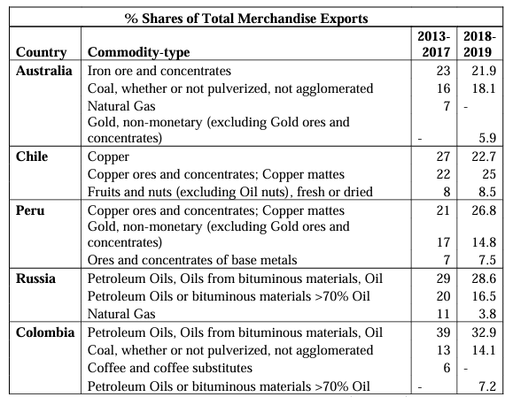
In the selection of sovereign CDS data, we follow data published by UNCTAD (2019; 2021) “State of Commodity Dependence” reports and select the CDS of nations with flexible exchange rate regimes that are significant commodity exporters- thus allowing us to test how CToT shocks propagate through to sovereign risk in the view of financial market participants when exchange rates are flexible. Therefore, we use weekly OHLC data obtained from Thompson Reuters for the 5 Year CDS Spreads and FX rates (Australian Dollar, Peruvian Sol, Chilean Peso, Colombian Peso, and Russian Ruble) measured in units per US Dollar, and the relevant commodities for Australia, Peru, Chile, Colombia, and Russia (Table 1) obtained from ICE, COMEX, and CME. Our dataset runs from the 5th October 2012 to the 24th December 2021. We identify two categories of exporters which are Metals exporters including Australia, Peru, and Chile, and those that are Oil exporters which are Colombia and Russia. We also differ from the existing literature and 5 country-specific VARs to mitigate the effects of collinearity interfering with the model results as well as the manipulated GFEVDs. For example, Copper volatility could show as significant or volatility transmission to Australian CDS if we grouped all mining economies into one model, when this may be due to Iron and Copper being highly correlated as industrial metals.
In the metal exporting group, we select Iron and Gold for Australia, Copper and Gold for Peru, and Copper for Chile. We take a more simplistic approach for the energy economies and select the Oil price (Brent Crude benchmark) for Colombia and Russia. Moreover, we exclude Coal due to data limitations and Natural Gas in the Australian model due to being only marginally larger relative to Gold shown across the UNCTAD full dataset where the latter may yield interesting results due to its “safe haven” status in the financial-economic literature (Baur & Mcdermott, 2016). Although this may add concern for omitted variable bias in the Australian and Colombian models, these are not the largest exports and should only affect the results of our VAR models rather than the GFEVDs. The inclusion of Gold prices in the Australian model also helps to mitigate this and accounts for more commodity exposure.

VOLATILITY CALCULATIONS
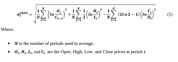
Calculating the logarithmic returns of assets (in this case CDS spreads and Commodity indices) is of course trivial, but with realised volatility, this is not the case. Parkinson (1980) demonstrates how simplistic close-close estimation is inferior to that of another which utilises the high and low data of the given period, developing an estimator 5.2 times more efficient than close-close. Indeed, Diebold and Yilmaz (2012) adopt this estimator, and Alizadeh et al. (2002) find that “theoretically, numerically, and empirically that range-based volatility proxies are not only highly efficient but also approximately Gaussian and robust to microstructure noise”. This approach, however, fails to account for market movements after the market close, presenting a bias of underestimation. Garman and Klass (1980) solve this problem by extending the formula and including the open and close price of a given asset subsequently achieving 7.4 times efficiency on close-close. Rogers and Satchell (1991) incorporate drift, for when the underlying average log return is not equal to zero achieving 8 times the efficiency of close close estimation. Yang and Zhang (2000) then extend the Garman and Klass (1980) model, to incorporate opening jumps and thus add more informational content achieving 8 times efficiency, and is the chosen volatility estimator for our model, hereafter referred to as GKYZ (Eq. 1). We use rolling 10-week average volatilities for our inputs into the model to smooth noise. Despite this class of volatility estimators being robust to microstructure noise, it should be noted that CDS spreads have notably low liquidity and are thus susceptible to randomness.

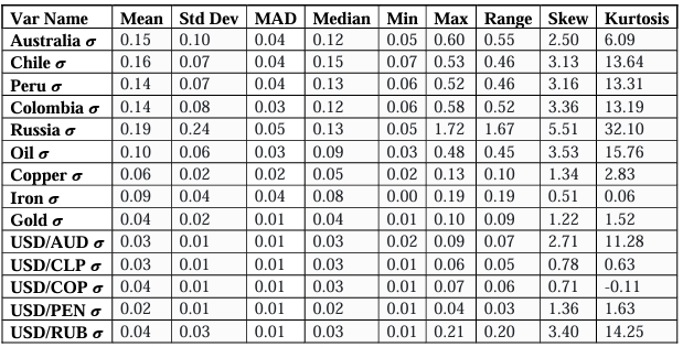
SUMMARY STATISTICS
Observing the summary statistics (Table 2), we see both the mean and median volatility of CDS spreads to be higher for all countries most likely due to these markets being significantly less liquid than those of commodities and the corresponding FX rates for each nation which are expectedly less volatile than the commodities themselves. As expected, the median Australian CDS volatility measure is significantly lower than that of Chile and Peru due to greater robustness in its economy and strong institutions but Australia’s CDS surprisingly has the second highest mean volatility in the as well as having a higher median than Colombian CDS volatility, potentially due to outlier effects. Using the Standard Deviation, we can also see that the volatility of volatility is greatest for Brazilian and Russian CDS, and the lowest for Peru and Chile CDS. We also observe high measures of kurtosis (>3) in the distributions across our dataset, indicating “fat tails” and non-normality, Copper, Iron, Gold, USD/CLP, USD/COP, and USD/PEN volatilities possess thinner tails with measures of (<3). The observation of non-normally distributed volatilities is also found in the skewness across most variables (<0 or >0). Therefore, the GKYZ formula failed to produce normal distributions.

6. METHODOLOGY
For our models, we utilise the framework by Diebold and Yilmaz (2012) in R Studio software due to the insights it generates on mean spillovers across our dataset as well as rolling spillovers generated across time. As such a framework is underpinned by GFEVDs from VAR models, we must specify our VAR models for each nation, which each contains K lags of 5 Year Sovereign CDS volatility for the nation, K lags of the corresponding Foreign Exchange rate volatility, and K lags of the volatility for at least one commodity that the country exports. An example specification as a trivariate VAR (1), for a given country with only one commodity and K = 1 lags is provided (Eq. 2).
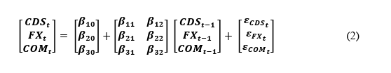

Where:
• 𝑪𝑫𝑺𝒕 is the 5 Year CDS Spread volatility for a given country.
• 𝑭𝑿𝒕 is the Foreign Exchange rate volatility for a given country.
• 𝑪𝑶𝑴𝒕 is the volatility of the Commodity the given country is dependent on.
• 𝜷𝟏𝟎, 𝜷𝟐𝟎, 𝜷𝟑𝟎 are vector constants.
• All other 𝜷𝟏𝟏, 𝜷𝟏𝟐, 𝜷𝟐𝟏, 𝜷𝟐𝟐, 𝜷𝟑𝟏, and 𝜷𝟑𝟐 are the matrix coefficients for the
column vector(s) of independent variables.
As previously discussed, the essence of the framework is to essentially manipulate the KPPS GFEVDs from each VAR to construct metrics of volatility spillovers in both various aggregated measures as well as pairwise measures. In this paper, we generate pairwise results for the full sample, in addition to a sample that excludes the financial market shock induced by COVID-19. In addition to this, we construct rolling Net Total Spillovers across our models so that we can study how spillovers are transmitted from particular assets across time. For our models, we generate the GFEVDs from a two-step-ahead forecast, and more generally, Diebold and Yilmaz (2012) calculate the H-step-ahead GFEVD (Eq. 3).
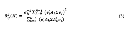

Where:
• 𝒆𝒋 is an m x 1 selection vector with unity as its jth element and zeros elsewhere; and
e′i is its transposed variant.
• 𝒆𝒊 is an m x 1 selection vector with unity as its ith element and zeros elsewhere.
• 𝑨𝒉 is a coefficient matrix for h steps ahead and 𝑨’𝒉 is its transposed variant.
• 𝝈𝒋𝒋 is the standard deviation of the error term for the jth equation.
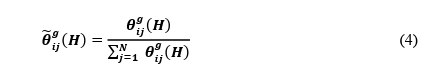
It should be noted however that because the underlying Generalised KPPS VAR assumes simultaneity in shocking variables and analysing the contemporaneous correlations, as highlighted by Pesaran and Shin (1998), the shocks from and to a given variable (the row sum) do not sum to unity (100%) of all shocks. Arising from this is a problem of interpretation when conducting our analysis, we may be able to claim which shocks to and from a given variable are the largest however this does not tell us the proportion of the total forecast error variance such shocks account for. A common adjustment made is to normalise each shock by the row sum of the shocks, thus providing us with a percentage of the contribution to the total forecast error variance of a given variable. For example, Lanne & Nyberg (2016, pp. 4) similarly modify the GFEVD to solve the problem posed by the nature of the KPPS Generalised VAR by “aggregating the cumulative effect of all the shocks while the numerator is the cumulative effect of the ith shock”. Diebold and Yilmaz (2012) solve the issue as follows (Eq. 4).

Now the interpretation problem has been mitigated, the spillover indices can then be constructed. To start with, the Total Spillover index can be constructed (Eq. 5), which is the generalised variant of that seen in Diebold and Yilmaz (2009).
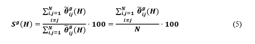

The Total Spillover index measures the influence of all spillovers across time on the total forecast error variance of the specified model, thus indicating how widespread volatility transmission is across the asset markets under examination, in this case, how widespread volatility transmission is across the CDS spreads of a particular class of commodity export dependent Emerging Markets, as well as the relevant commodity index. This, however, does
not provide us with a directional assessment of such spillovers, and therefore we describe the novel spillover indices unique to the Diebold and Yilmaz (2012) framework, beginning with the directional total spillovers. This provides a measurement of the spillovers received by market i from all other markets j (Eq. 6). Similarly, the directional total spillovers transmitted by market i to all other markets j can be calculated (Eq. 7).
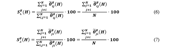

The results of this are not of particular interest, however, as it is the net direction which ultimately matters for our analysis, but we can use such a metric to calculate the net (directional) total spillovers. We use this metric both averaged over the dataset as well as being studied across time using 52-week rolling window estimation, which allows us to gauge where Net Transmission originates in the systems at any one time. Therefore, we can calculate the Net Total Spillovers from a market i to all other markets j (Eq. 8).
![]()

The most significant of manipulated GFEVD metrics is that of the Net Pairwise spillovers which provide us with the direction of net volatility transmission between two asset markets, which is crucial to validate our economic hypotheses. Unfortunately, due to technological limitations, we are unable to compute a time-varying metric for Net Pairwise spillovers as can be done with Directional Total spillovers. Although this is true, we remain able to compute the metric averaged across time through the observation and computation from the generalised spillover table which provides us with another base to answer our economic hypotheses. The metric is specified as the spillovers transmitted by an asset market j to another asset market i on a net basis (Eq. 9).

7. MODELS & RESULTS
For each commodity-exporting nation, we use two VARs, one which includes a dataset excluding the effects of COVID-19 from the 5th October 2012 to the 27th December 2019, and another which includes the effects of COVID-19 from the 5th October 2012 to the 24th December 2021. This approach is utilised to help us disentangle the COVID-induced shock to commodity prices and other assets in the models for Net Pairwise Spillovers and compare them with our rolling Net Total Spillovers. For simplicity, we only highlight diagnostics, VAR
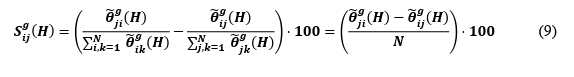
summaries, and Net Total Spillovers for the full sample of data. Before specifying our VAR models, it is first crucial to test for the optimal selection of lags for each commodity class VAR. We achieve this using a lag selection process where VARs are estimated by OLS per equation, and we compute various information criteria to then compare which lags produce the minimal score amongst the different criteria (Table 3). These include those of Akaike’s Information Criterion (AIC), Hannan-Quin (HQIC), Schwarz Criterion (SIC), and the Final Prediction Error Criterion (FPE). We test for a maximum of 12 lags. AIC penalises a model for having more estimators relative to its performance but assumes that none of the models estimated is true, and that reality has far greater dimensionality. FPE is also closely related to AIC as both test the models on another dataset, which is the mechanism through which both measures of fit assume none of the tested models is true. SIC, however, assumes that one of the model orders is the true model. The SIC along with HQIC is stricter than AIC in penalizing more parameters. Koehler and Murphree (1998) conclude that SIC is favourable as AIC and FPE tend to overfit data and lead to relative over-parametrization. For consistency, we, therefore, use SIC for lag selection and use the same lags for our pre-COVID sample models. We test a maximum of 12 lags for each country-specific VAR model and use judgement when significant discrepancies arise between SIC and other criteria, increasing the lag order by 1. Therefore, we select 2 lags for the Australia and Peru models, 3 lags for the Chile model, and 10 lags for the Colombia and Russia models.

We then perform several diagnostics tests on our models. After discovering unit roots in our variables, we take their first differences and reject the hypothesis of unit roots being present at the 1% level, except for the eighth, eleventh, and twelfth lags of Iron volatility which were significant at the 5%, 5% and 10% levels respectively (Appendix 1). The VAR stability tests (Appendix 2 & 3), also show that our models are stable using both a generalised dynamic empirical fluctuation test (Kuan & Hornik, 1995) and by observing that the modulus of the eigenvalues are strictly less than one. This is the most important consideration to ensure that the stochastic shocks captured in the GFEVDs do not persist. The Jarque-Bera tests for normality also confirm the results of the descriptive statistics, showing all model residuals are not characteristic of a normal distribution (Appendix 4). For serial correlation it can be shown by using the Breusch-Godfrey tests (Appendix 5) that the optimal lags selected by the SIC results were not sufficient in capturing the full autoregressive process (aside from the Chile model at 6 lags), we attribute this to the rolling-average volatilities used as greater lag orders did not fail to reject the null hypothesis of no serial correlation. This may not be so serious as the rolling averages still capture the data up to 10 lags. Results from the multivariate ARCH-
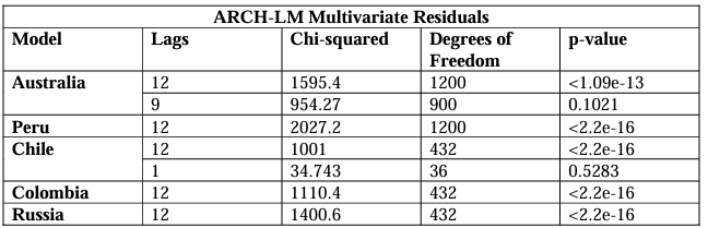
LM tests (Appendix 6) show rejections of the null hypothesis of no heteroskedasticity and that our GKYZ metrics failed to capture all the heteroskedasticity in the security prices except for the Australia model which captures up to 9 lags, and the Chile model at only 1 lag. These results show our models are not as efficient as they could be, biasing standard errors and therefore the significance of our variables. Despite not being able to robustly confirm the significance of the model variables, we assess the overall pattern of p-values across our five models as well as the parameter signs. Moreover, our parameter estimates are still linear and unbiased so we may conclude that our model results are suitable for analysis (except for non normality) within the context of volatility spillovers, the focus of this investigation.
VAR RESULTS
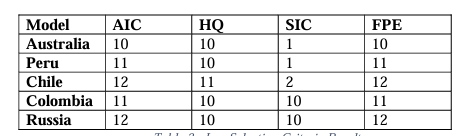
Beginning with Australia (Table 4) in the Metals exporting economies, in explaining the CDS volatility, only the first and seconds lags of the dependent variable itself are significant at the10% and 1% levels respectively and no other variables- with the parameter coefficients of both lags expectedly positive. Despite not being significant, both Iron volatility lags and the second for Gold were estimated to be mildly negative overall with the FX volatility lags being overwhelmingly positive. The first lag of Gold price volatility is however significant at the 5% level and the second at 10% in explaining the volatility of FX and was expectedly positive- in addition to the first lag of FX volatility at 1% significance also positive. Iron volatility was again insignificant and failed to explain FX volatility.
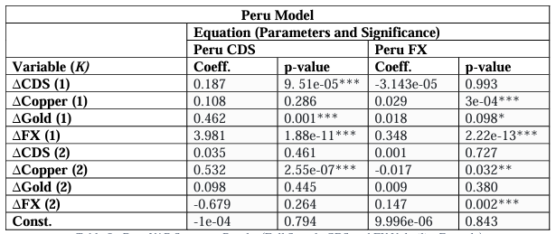
For Peru however (Table 5), the first lags of both FX and Gold volatility and the second for Copper volatility are significant at the 1% level in explaining the CDS volatility of Peru. The estimated parameter coefficients are also expectedly positive for these variables, signalling an overall confirmation of the hypotheses. Additionally, the first lag of Copper volatility is significant at 1%, the first lag of Gold volatility at 10%, and the second lag of Copper at the
5% level in explaining the volatility of FX (as well as the first and second lags of the dependent
variables themselves significant at 1%). Unsurprisingly, the first and second lags of FX
volatility are positive, the first (positive) lag of Copper volatility is also considerably larger in
absolute terms than the second (negative) lag with both lags of Gold being positive- despite the
second being insignificant.
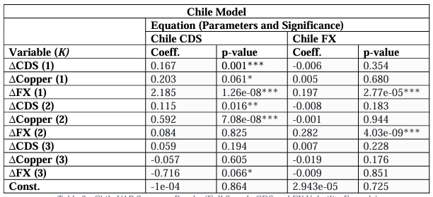
In the model summary for Chile (Table 6), we again see both the volatility of the commodity that the country depends on, as well as the nation’s exchange rate explaining the movement in Chile’s CDS spread volatility with the first and second lags of Copper significant at 10% and 1% respectively, whilst the second and third lags of FX volatility were significant at 1% and 10%, in addition to lags one and two of the dependent variable itself, being significant at 1% and 10% respectively. Although this is true, the third lag of FX volatility is surprisingly negative, though overwhelmingly outweighed by the positive effect of the first- all other significant parameter coefficients were estimated as positive as one would expect. Interestingly, the finding that the FX volatility is a significant predictor of CDS volatility for Chile and Peru but not for Australia is consistent with the financial literature that Emerging Markets are particularly susceptible to currency crises shocking the economy as well as generally less competent and less robust Central Banks. Surprisingly, the Copper price volatility was not at all significant in explaining the volatility of FX and as expected neither were any of the lags for the nation’s CDS volatility. The first two out of the three lags for the dependent variables were positive and significant at the 1% level.


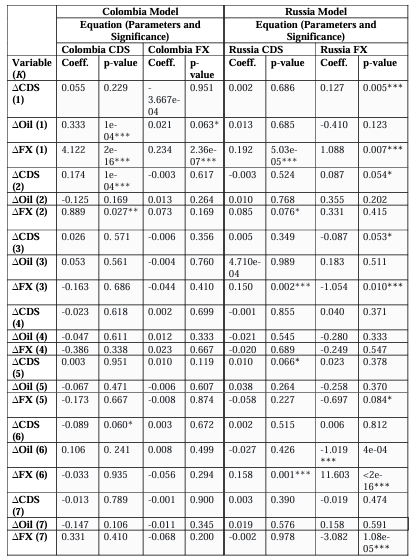
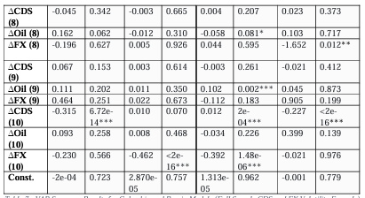
Turning to the group of Oil export-dependent nations, we begin with the VAR model for Colombia (Table 7, LHS). We find that as expected, both Oil and FX volatilities help explain the volatility in Colombian CDS with the first lag of Oil positive and significant at 1% and the first and second lags of FX volatility being positive and significant at 1% and 10% levels respectively. Additionally, the lags of the second, sixth and tenth CDS volatilities are significant at the 1%, 10%, and 1% levels respectively however the sixth and tenth lags were surprisingly negative. The results of the equation for Colombian FX are more mixed, however. Lag one of Oil volatility is significant at the 10% level as expected and both the first and tenth lags of FX volatility are significant at the 1% level, but we unexpectedly find the tenth lag of CDS volatility to be significant at the 1% level. The tenth FX lag is unexpectedly negative but
when observing all parameter estimates across the board, the coefficient signs are mixed which is likely given such a large number of lags.
For the Russian model (Table 7, RHS) in the equation for Russia’s CDS volatility, we also find mixed results for the parameter signs. We find the eighth and ninth lags of Oil volatility to be significant at 10% and 1% with the ninth lag’s absolute size far outweighing the negativity of the eighth. Additionally, the first, second, sixth, and tenth lags of the FX volatility were positive overall and significant at the 1% level and the third at the 10%. We also find the fifth and tenth lags of the dependent variable were positive and significant at the 10% and 1% levels respectively. In the equation for Russian FX volatility, we find that the sixth lag of Oil is significant at 1% but is negative, and bizarrely, CDS volatility contained some explanatory power. The first and tenth lags are significant at 1%, whilst the second and third, are significant at 10% which may be possible due to such lags having absorbed previous information in the exchange rate. Although this is true, explanatory power is most overwhelmingly driven by the dependent variable with the size of its coefficients being relatively much larger, with the sixth lag having a particularly large parameter estimate. We find the first, third, sixth, and seventh significant at 1% and the eighth at 10%.


VOLATILITY SPILLOVER RESULTS
Following the discussion of the results from the country-specific VARs and how our parameter estimates compare with our expectations, we now turn to the primary findings of the paper, analysing the volatility spillovers between CDS Spreads, Commodities, and FX. We achieve this by looking at how the manipulated GFEVDs show whether a variable is a Net Total transmitter or receiver of volatility in the system on both a mean and rolling window basis in addition to the Net Pairwise spillovers of volatility to further bolster our analysis at a more granular level. Unlike the significance of the model parameters, the results are relatively robust to the detected inefficiencies except for normality, which the GFEVD calculations assume.
AUSTRALIA
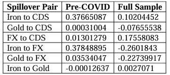
Beginning with those of the Australia model (Table 8), we find as expected that Australian CDS is a net receiver of volatility spillovers, but that Iron volatility is unexpectedly a net receiver of spillovers, Gold volatility is a significant receiver in the system, and that FX is a net transmitter of volatility highlighting that it is the key driver of volatility in the system. Examining the Net Pairwise spillovers (Table 9) from the full sample, Iron price volatility expectedly spills into Australian CDS volatility but Australian CDS volatility spills into Gold price volatility, and the FX volatility spills into both the Australian CDS and Gold volatilities on a net basis. Pre-COVID, the same relationships existed however Gold was a near-zero transmitter and the spillovers from FX to CDS were significantly lower. Interestingly, the results highlight the significance of Iron exports relative to those of Gold in the role of sovereign risk and that Gold may be a major receiver due to its “safe haven” status during the presence of macroeconomic uncertainty. Despite this, Iron volatility was a net transmitter to FX as expected, but an unexpected receiver following the shock induced by COVID.

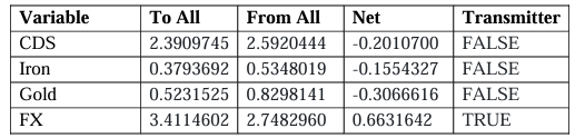

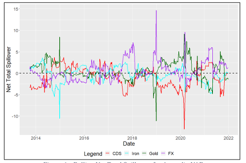
As can be seen from our rolling Net Total spillovers (Figure 1), it is very clear that Australian CDS volatility, on average, is a net receiver of volatility spillovers amongst other variables, and the model correctly captures this at the beginning of the COVID pandemic, but surprising not during the late 2014 commodity crisis. The same is true for the net transmission of FX volatility also, which is not seen during late 2014 but is seen sharply as COVID-19 volatility occurs. Consistent with our full sample mean Net Total spillover table, we also see Iron surprisingly being a net receiver of volatility during both crises in the system, but bizarrely see Gold being a net transmitter, particularly as both the late 2014 commodity crisis and COVID 19 shock occurs.

PERU
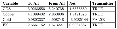
For the manipulated GFEVDs from the Peru model, we also find some mixed results with the Copper price volatility expectedly being a net transmitter as well as the volatility of FX, but then find the CDS Volatility of Peru unexpectedly being a net transmitter in the system in addition to the Gold price volatility being a net receiver (Table 10). Examining the Net Pairwise results (Table 11), we find that Copper is expectedly a net transmitter to Peru CDS and FX volatility, though as in the Australia model, the spillovers to CDS volatility are lesser in the full sample than they are pre-COVID surprisingly. We also find that Gold is a Net Pairwise receiver of spillovers from Copper and Peru CDS volatility (and this intensifies with the COVID pandemic), but is a net transmitter to FX which decreases with the emergence of COVID. This is an interesting observation for Gold volatility as despite being a component of Peru’s exports, spillovers from Copper and CDS volatility may reflect wider macroeconomic risk with Gold known as a “safe haven” asset during such periods. This does conflict with Gold transmitting to FX but we can see this decreases during COVID. Again, we find spillovers from FX being the largest amongst those to CDS, sharply increasing with the onset of COVID.


For the rolling Net Total spillover observations for Peru (Figure 2), we find an interesting set of results on the nation’s CDS volatility in that it shows particularly large spillovers to other asset volatilities within the system around the periods between 2015-2016, 2017-2018, and the beginning of 2020 through to the start of 2021. This aligns with the likelihood that coincident spillovers to Gold volatility are due to Gold’s “safe haven” status. Although Copper volatility begins to be a significant transmitter during the late 2014 commodity crisis, it quickly dips to be a net receiver where FX volatility instead appears to be the dominant transmitter to other variables (aside from CDS to Gold). Copper does however appear to be the dominant transmitter of volatility during the onset of the COVID-19 pandemic, with FX volatility being a net receiver of spillovers, presumably from Copper as the pairwise results would indicate. Although this is true, Copper appears to be a weaker pairwise transmitter of volatility over COVID-19 so we deduce the remainder of net transmission to be a signal of macroeconomic
uncertainty to Gold.

CHILE
Observing the results from the GFEVDs in the Chile model, we find that as expected, Chilean CDS volatility is a net receiver of volatility in the system (by a large margin), with both the volatility of Copper and FX markets being net transmitters of volatility (Table 12). Looking at the pairwise results (Table 13), we find that both Copper market and FX volatilities are transmitters to Chilean CDS volatility, with FX being the dominant transmitter intensifying and Copper marginally weakening in the full sample with the COVID pandemic. Interestingly, the results do not show Copper being a Net Pairwise transmitter to the FX volatility and instead show the contrary which diminishes to near zero with COVID included in the sample.


For Chile’s rolling Net Total spillovers (Figure 3), we see the Chilean Peso volatility being a significantly greater transmitter of volatility than seen in the currencies of Australia and Peru. We do generally see the Chilean CDS volatility being a net receiver of volatility as expected with some brief periods of net transmission to other variables in the system. During the COVID-19 crisis, we see CDS volatility spillovers rising sharply in an unexpected manner followed by a fall in volatility spillovers from the Chilean Peso into negative territory along with a sharp reaction from Copper volatility spillovers turning negative. Interestingly, during the global commodity crisis of late 2014, we see net spillovers from Copper volatility rise sharply, far into the positive territory whilst both the Chilean CDS and Peso volatility fall which signifies the crash in prices negatively affected the currency and the nation’s CDS.

COLOMBIA
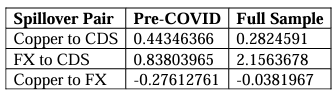
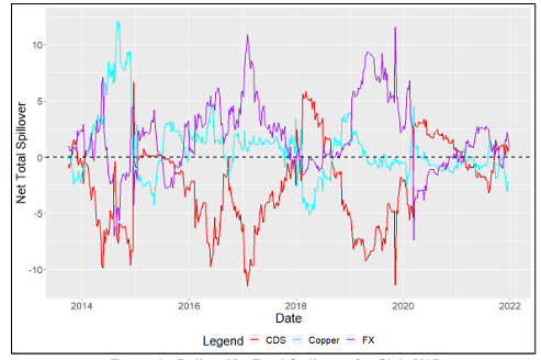
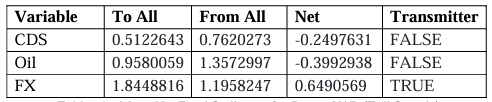
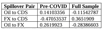
Now turning to the energy group of models, we find that as expectedly within the Colombian VAR system, the GFEVDs display Colombian CDS volatility being a net receiver of spillovers, Oil volatility being a net transmitter, and the FX volatility being a net transmitter of volatility within the system (Table 14). We find slightly negative Net Pairwise spillovers (Table 15) from Oil volatility to that of Colombian CDS until the COVID-19 pandemic is included in the full sample, where spillovers flip to being positive and of a significant magnitude. Additionally, we see even larger volatility spillovers from the Colombian Peso to the Colombian CDS volatility which intensify during COVID-19. The former finding is contrary to that of Bouri et al. (2017) who find significant spillovers in their full sample from the overall commodity index to Colombia or in the energy sub-index. Interestingly, Oil volatility did not spill over into FX volatility and instead the contrary is found to be true over both time horizons, becoming more negative during COVID.


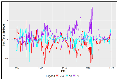
Rolling Net Total spillover results for Colombia (Figure 4) indicate strong alignment with our set of economic hypotheses across the full sample. Overall, we have seen an overwhelmingly negative spillover in Colombian CDS volatility signifying it was a receiver from other assets with the largest receipt of volatility being during the COVID-19 pandemic. Surprisingly, the spillover from Oil Volatility to the rest of the system during the Commodity crisis of late 2014 was very brief before dipping to become a net receiver of spillovers, and the volatility of the Colombian Peso was the strongest transmitter of volatility for a sustained period. For the shocks of the COVID-19 pandemic, however, it is very clear that both the volatility of Oil and the Colombian Peso was net transmitters of volatility to the volatility of Colombian CDS spreads. Following this, Oil volatility was a mild net transmitter with a short spike into receiving territory as global economies recovered into 2021 and 2022 (with some periodic lockdowns) and demand for commodities spiked which accompanied the structural under-supply of Oil.

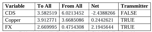
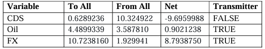
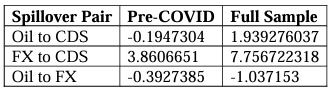
RUSSIA
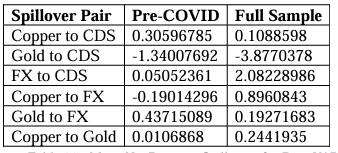
In the Russia model, we see that as expected, Russian CDS volatility is a net receiver of volatility within the system, however, Oil volatility is detected as a net receiver which is surprising given Russia’s dependence on Oil exports. Of all assets, the volatility of the Ruble was the standalone net transmitter by a large margin (Table 16). Turning to the Net Pairwise spillovers (Table 17) we see that CDS volatility is impacted by spillovers from FX volatility as expected but only when COVID-19 is included and was flipped from being a relatively large receiver in the sliced sample. Oil as expected was a net transmitter to CDS in the pre-COVID but then surprisingly flips to being a net receiver in the full sample. This particular result aligns with that of Bouri et al. (2017) who find no significant spillovers in their full sample for the energy market index to Russian CDS as well as that of Cheuffart and Hooper (2019) with FX volatility being dominant in volatility spillovers to Russian CDS. Although this is true, Bouri
et al. (2019) find that energy market volatility does affect Russian CDS volatility but only in the middle and upper quantiles. Moreover, we expectedly see Oil being a net transmitter to FX pre-COVID but surprisingly, we see Oil being a net receiver in the full sample.


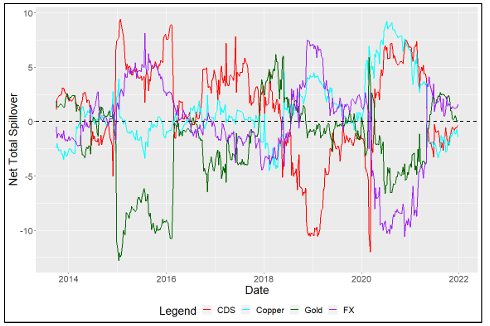
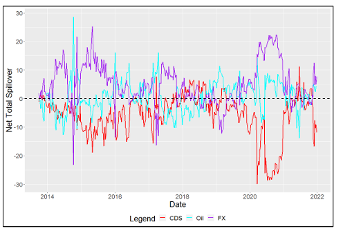
The rolling Net Total spillovers from the Russian VAR system (Figure 5) render another set of interesting results. Whilst the CDS spread volatility again overwhelming remains as a receiver of volatility spillovers as expected, the 2014 commodity crisis led to a sharp rise in spillovers from Oil volatility as one would expect, but then sharply and briefly dips under the negative zone to become a mild receiver of spillovers. FX was briefly a receiver of volatility spillovers during late 2014 and then became a strong transmitter to the rest of the system. Continuing on from this, there was the Russian Financial Crisis lasting until around 2016 with large net spillovers to Russian CDS volatility just after. The model shows a prominent transmission from FX and Oil volatility presumably to the volatility of Russian CDS during the crisis. At the start of the COVID-19 pandemic, the results show the Oil volatility being a net receiver along with CDS. FX volatility was again, an overwhelmingly large net volatility transmitter throughout the period. As the Russian economy recovered (with periodic lockdowns) we see also see spikes in net FX volatility transmission and the net receipt of volatility for CDS, particularly at the end of 2021.

8. DISCUSSION
After summarising our VAR results, we find common patterns across models, most notably with FX volatility being significant in explaining CDS volatility in all models except that for Australia, which we attribute to the relative strength of its economy and central banks. Key export commodity volatility is significant in explaining volatility in most of our models except for Australia and Colombia. In the FX equations as we hypothesised commodity volatility was found to be significant in the models for Australia (except for Iron), Peru, and Russia. Surprisingly, we find that CDS volatility was significant in explaining FX volatility in the Colombia and Russia models.
We observe mixed results from our manipulated GFEVDs owing to averaged Net Total spillover metrics expectedly aligning with our hypotheses, which is that CDS spread volatility is typically a receiver of volatility transmission except for Peru, which we attribute to its pairwise net transmission to Gold due to its financial “safe haven” status. We also find that commodity price volatility is typically a net transmitter across the systems, except for in the
Australia and Russia models. Moreover, we find nominal FX volatility to be the key driver of volatility across all systems, possibly due to the overrepresentation of Emerging Markets in our study. We also use 52-week rolling window spillovers to analyse the Net Total volatility spillovers for each variable in each country’s VAR system so that we can analyse such spillovers across the time series to further contextualise the results within recent economic and financial market history. Two of the most vivid events throughout our time series are the Commodity Price Crisis of late 2014 and the 2020 COVID-19 pandemic. By relating the Net Total spillover movements to their averages across the full sample as well as the Net Pairwise spillovers, we also deduce that such movements highlighted occur across those two notable events. The Net Pairwise results are mixed across the board in aligning with our hypothesis that commodity volatility will cause volatility in an exporter’s CDS spread, with some surprising results generated on our pre-COVID and full sample models. For example, for Australia, Peru, Chile and Colombia the largest commodity export price volatilities (Iron, Copper, Copper, and Oil respectively) transmit to the relevant CDS volatilities but in the case of the former three countries, the spillover surprisingly decreases with COVID-19 included (in the full sample). Only the Russia model and the Gold transmission dynamic in the Australia and Peru models support this hypothesis and in the case of the latter, we find the Gold “safe haven” status dominating the transmission (with increasing intensity with the occurrence of COVID) in financial markets rather than the CToT significance of the commodity. Moreover, we see the pairwise net volatility transmission from FX to CDS across all models other than that for Russia in the pre-COVID sample, with this spillover intensifying in the COVID-included full sample across all VAR models- as we would expect given the intense negative demand shock coupled with the vast monetary response across the globe. These Net Pairwise spillovers in addition to the Net Total spillovers from FX align with the findings of Feng et al. (2021) who find Net Pairwise spillovers from FX to CDS markets, especially among Emerging Markets. Such nations typically possess poorer institutions and central bank governance. These institutional factors may also explain that despite each country having flexible exchange rates, financial markets still perceive export CToT shocks materially affecting sovereign risk across most of the countries studied in this paper. We also found mixed results for the Net Pairwise transmission from commodities to FX (the hypothesised shock absorber) with the picture being unclear of how the commodity volatility spillovers transmit (via FX) into CDS volatility in our results. In future papers, insights could be provided through secondary cross-sectional analyses of the spillover results, so that institutional factors can be statistically tested for their significance in explaining the spillovers, along with the type of commodity, and other factors.
9. CONCLUSION
We contribute to the existing applied literature using the Diebold and Yilmaz (2012) framework as the first paper that uses standard volatility spillovers between commodities, foreign exchange rates, and sovereign CDS spreads as opposed to more complex methods such as the extreme spillover approaches (Cheuathonghua et al., 2022), especially where the coverage of the COVID-19 pandemic is concerned. The analysis also involves the use of an alternative calculation of historical volatility for these assets, which is closely related to, but not yet used in the existing literature and includes the variables relevant to each country in their own specific VARs, an approach that has not yet been taken in this specific context. Due to the complex nature of financial market dynamics, we propose other studies use a wider set of data where possible. This could include a comparison of historical volatility models as inputs, import relevant commodities, different types of volatility spillovers (extreme or normal), asymmetric volatility effects, and those economies which have fixed exchange rates so that subsequent cross-sectional analysis can be undertaken to understand further the role of institutions and currency regimes in dictating the volatility spillovers between commodities, FX, and CDS spreads. Therefore, we see a wide scope of potential extension for this topic in the future. Though it was not the sole focus of our study, standard errors robust to serial correlation or heteroskedasticity should also be used so that subsequent tests can be undertaken to greater understand the statistical significance, and to compare results between fixed and flexible exchange rate regimes that are commodity export dependent.
10. REFERENCES
• Alizadeh, S., Brandt, M. and Diebold, F., 2002. Range-Based Estimation of Stochastic Volatility Models. The Journal of Finance, 57(3), pp.1047-1091.
• Alsadiq, A., Bejar, P. and Otker-Robe, I., 2022. Commodity Shocks and Exchange Rate Regimes: Implications for the Caribbean Commodity Exporters. IMF Working Papers, (2021/104).
• Ampofo, G., Jinhua, C., Bosah, P., Ayimadu, E. and Senadzo, P., 2021. Nexus between total natural resource rents and public debt in resource-rich countries: A panel data analysis. Resources Policy, 74, 102276.
• Auty, R., 1993. Sustaining Development in Mineral Economies: The Resource Curse Thesis. 1st Edition. Routledge, London.
• Baur, D. and McDermott, T., 2016. Why is Gold a safe haven?. Journal of Behavioral and Experimental Finance, 10, pp.63-71.
• Ben Zeev, N., Pappa, E. and Vicondoa, A., 2017. Emerging economies business cycles: The role of commodity terms of trade news. Journal of International Economics, 108, pp.368-376.
• Bollerslev, T., 1987. A Conditionally Heteroskedastic Time Series Model for Speculative Prices and Rates of Return. The Review of Economics and Statistics, 69(3), pp.542-547.
• Bollerslev, T., 1990. Modelling the Coherence in Short-Run Nominal Exchange Rates: A Multivariate Generalized Arch Model. The Review of Economics and Statistics, 72(3), pp.498-505.
• Bouri, E., de Boyrie, M. and Pavlova, I., 2017. Volatility transmission from commodity markets to sovereign CDS spreads in emerging and frontier countries. International Review of Financial Analysis, 49, pp.155-165.
• Bouri, E., Jalkh, N. and Roubaud, D., 2019. Commodity volatility shocks and BRIC sovereign risk: A GARCH-quantile approach. Resources Policy, 61, pp.385-392.
• Broda, C. and Tille, C., 2005. Coping with Terms-of-Trade Shocks in Developing Countries. Federal Reserve Bank of New York – Current Issues, 9(11)
• Brownlees, C.T., Engle, R., & Kelly, B. (2011) A practical guide to volatility forecasting through calm and storm. The Journal of Risk. 14. pp. 3-22.
• Cheuathonghua, M., de Boyrie, M., Pavlova, I. and Wongkantarakorn, J., 2022. Extreme risk spillovers from commodity indexes to sovereign CDS spreads of commodity dependent countries: A VAR quantile analysis. International Review of Financial Analysis, 80, 102033.
• Chuffart, T. and Hooper, E., 2019. An investigation of Oil prices impact on sovereign credit default swaps in Russia and Venezuela. Energy Economics, 80, pp.904-916.
• Dauvin, M., 2016. Sovereign spreads in emerging economies: do natural resources matter? EconomiX Working Papers 2016-11, University of Paris Nanterre, EconomiX
• Diebold, F. and Yilmaz, K., 2008. Measuring Financial Asset Return and Volatility Spillovers, with Application to Global Equity Markets. The Economic Journal, 119(534), pp.158-171.
• Diebold, F. and Yilmaz, K., 2012. Better to give than to receive: Predictive directional measurement of volatility spillovers. International Journal of Forecasting, 28(1), pp.57 66.
• Diebold, F. and Yılmaz, K., 2014. On the network topology of variance decompositions: Measuring the connectedness of financial firms. Journal of Econometrics, 182(1), pp.119 134.
• Engle, R. F., & Kroner, K. F. (1995). Multivariate Simultaneous Generalized Arch. Econometric Theory, 11(1), pp.122–150.
• Engle, R., 1982. Autoregressive Conditional Heteroscedasticity with Estimates of the Variance of United Kingdom Inflation. Econometrica, 50(4), pp.987-1007.
• Engle, R., 2002. Dynamic Conditional Correlation. Journal of Business & Economic Statistics, 20(3), pp.339-350.
• Engle, R., Ito, T. and Lin, W., 1990. Meteor Showers or Heat Waves? Heteroskedastic Intra-Daily Volatility in the Foreign Exchange Market. Econometrica, 58(3), pp.525-542.
• Feng, Q., Sun, X., Liu, C. and Li, J., 2021. Spillovers between sovereign CDS and exchange rate markets: The role of market fear. The North American Journal of Economics and Finance, 55, 101308.
• Fernández, A., Schmitt-Grohé, S. and Uribe, M., 2017. World shocks, world prices, and business cycles: An empirical investigation. Journal of International Economics, 108, pp.S2-S14.
• Fornero, J., Kirchner, M. and Yany, A., 2022. Terms of trade shocks and investment in commodity-exporting economies. Repositorio Digital Banco Central.
• Garman, M., & Klass, M. J. (1980). On the Estimation of security price volatilities from historical data. The Journal of Business, 53, pp.67–78
• Ghecham, M., 2020. Further attempt to explain the Oil curse mechanism using a debt overhang concept. Journal of Economic Studies, 48(4), pp.852-868.
• Hooper, E., 2022. Oil and Gas, which is the Belle of the Ball ? The Impact of Oil and Gas Reserves on Sovereign Risk. Working Papers halshs-01211506, HAL.
• Hyeongwoo, K., 2009. Generalized Impulse Response Analysis: General or Extreme? Munich Personal RePEc Archive.
• Kaminsky, G., 2022. Terms of Trade Shocks and Fiscal Cycles. NBER Working Paper Series, No. w15780, pp. 1-16.
• Koehler, A. and Murphree, E., 1988. A Comparison of the Akaike and Schwarz Criteria for Selecting Model Order. Applied Statistics, 37(2), pp.187-195.
• Koop, G., Pesaran, M. and Potter, S., 1996. Impulse response analysis in nonlinear multivariate models. Journal of Econometrics, 74(1), pp.119-147.
• Kose, M., 2002. Explaining business cycles in small open economies. Journal of International Economics, 56(2), pp.299-327.
• Kuan, C. and Hornik, K., 1995. The generalized fluctuation test: A unifying view. Econometric Reviews, 14(2), pp.135-161.
• Lanne, M. and Nyberg, H., 2016. Generalized Forecast Error Variance Decomposition for Linear and Nonlinear Multivariate Models. Oxford Bulletin of Economics and Statistics, 78(4), pp.595-603.
• Mendoza, E., 1995. The Terms of Trade, the Real Exchange Rate, and Economic Fluctuations. International Economic Review, 36(1), p.101.
• Parkinson, M., 1980. The Extreme Value Method for Estimating the Variance of the Rate of Return. The Journal of Business, 53(1), p.61-65.
• Pesaran, H. and Shin, Y., 1998. Generalized impulse response analysis in linear multivariate models. Economics Letters, 58(1), pp.17-29.
• Restrepo-Echavarria, P., Mendoza, E. and Hamann, F., 2018. Resource Curse or Blessing? Sovereign Risk in Resource-Rich Emerging Economies. FRB St. Louis Working Paper No. 2018-32
• Robinson, J., Torvik, R. and Verdier, T., 2006. Political foundations of the resource curse. Journal of Development Economics, 79(2), pp.447-468.
• Roch, F., 2019. The adjustment to commodity price shocks. Journal of Applied Economics, 22(1), pp.437-467.
• Rogers, L. C. G., & Satchell, S. E. (1991). Estimating variance from high, low and closing prices. The Annals of Applied Probability, 1, pp.504–512
• Schmitt-Grohé, S. and Uribe, M., 2018. How important are terms-of-trade shocks? International Economic Review, 59(1), pp.85-111.
• Sun, X., Wang, J., Yao, Y., Li, J. and Li, J., 2020. Spillovers among sovereign CDS, stock and commodity markets: A correlation network perspective. International Review of Financial Analysis, 68, 101271.
• Tse, Y. and Tsui, A. (2002) A Multivariate GARCH Model with Time-Varying Correlations. Journal of Business and Economic Statistics, 20, pp.351-362.
• UNCTAD, 2019. The State of Commodity Dependence 2019. [online] https://unctad.org/webflyer/state commodity-dependence-2019
• UNCTAD, 2021. The State of Commodity Dependence 2021. [online] https://unctad.org/webflyer/state commodity-dependence-2021
• Wang, X., Xu, W. and Zhong, Z., 2018. Economic policy uncertainty, CDS spreads, and CDS liquidity provision. Journal of Futures Markets, 39(4), pp.461-480
• Yang, D. and Zhang, Q., 2000. Drift Independent Volatility Estimation Based on High, Low, Open, and Close Prices. The Journal of Business, 73(3), pp.477-492.
11. APPENDICES
Appendix 1 – Unit Root Tests

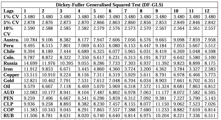
Appendix 2 – VAR Stability (Generalised Fluctuation Tests)

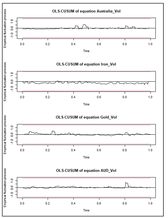

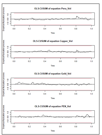

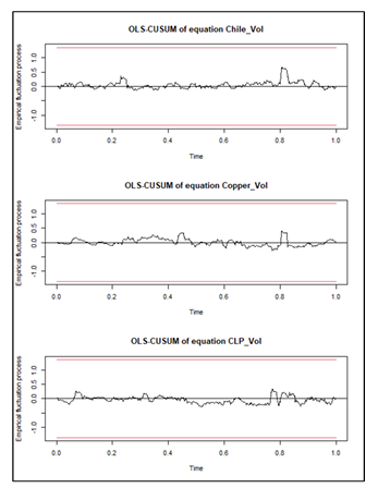

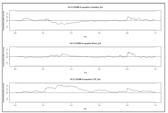

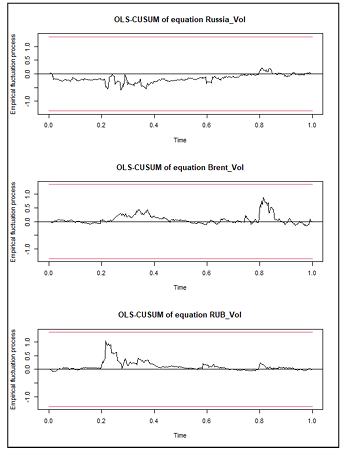
Appendix 3 – VAR Stability (Modulus of Eigenvalues)

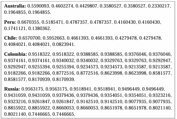
Appendix 4 – Normality Tests

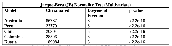
Appendix 5 – Serial Correlation

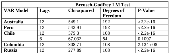
Appendix 6 – Heteroskedasticity Tests